11.1 FUNCTION SUBPROGRAMS

The FORTRAN language includes three types of functions: intrinsic functions, function statements, and function subprograms. Each of these types of functions calculates a single value. Intrinsic functions are built into the compiler and are directly accessible in a program. Statement functions and function subprograms allow the programmer to write needed functions that are not in the compiler's library. If the computation can be written in a single assignment statement the statement function should be used. A function subprogram is a complete, separate program from the main program that computes a single value that is returned to the main program in the function name. A function subprogram may contain any FORTRAN statement. It is composed of the function name, its argument list, a RETURN statement and an END statement. The general form is

type FUNCTION name (formal argument list)

FUNCTION name = value

RETURN

END

Example - Average of Three Numbers

c FORTRAN 77

c This program uses a function to find the average of three numbers.
        PROGRAM func_ave

c Type variables in main program (a, b, and c are local variables).
        REAL a,b,c,average

c Prompt for and get numbers to be averaged.
        PRINT *,'Enter the three numbers to be averaged.'
        READ *, a,b,c

c Invoke function average  
        PRINT *,'The three numbers to be averaged are ',a,b,c
        PRINT *,'The average of the three numbers is', average(a,b,c)
        STOP
        END

c Function average
        REAL FUNCTION average(x,y,z)

c Type variables in function (x, y, and z are local variables).
        REAL x,y,z

c Function name contains the value the function calculates and returns.
        average = (x + y + z)/3.0
        RETURN
        END

FORTRAN variables are local to their respective programs/subprograms. That is, they are accessible only by the program or subprogram in which they are defined. In the statement

PRINT *,`The average of the three numbers is ' , average(a,b,c)

the variables a, b, and c are local to the main program and are called the actual arguments. The values of a, b, and c are communicated to the function when it is invoked. In the function they are referenced by the local variables x, y, and z and are called the formal (because they give the form of the variable) or dummy arguments. The actual arguments and the formal arguments may have the same or different variable names.

The function name, average, holds the value of the average that is computed in the function.

An assignment statement, average = (x + y + z)/3.0, is used to store the average to be returned to the main program. The function name is part of an expression and may be placed anywhere an expression may be placed.

REAL FUNCTION average (x, y, z)

average = (x+y+z)/3.0

The argument list is the input values a, b, and c that the function needs to compute the average.

The type of the value returned, the average, is explicitly typed in the FUNCTION name

REAL FUNCTION average(x,y,z)

At the RETURN statement, control is returned to the main program where the function was invoked and program execution continues from that point.

The END statement indicates the end of the function.

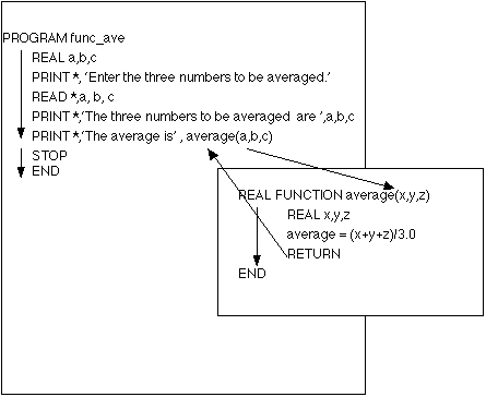
The sequence of execution of a main program and a function subprogram is given pictorially in Figure 1.

Figure 1

The gestation program in FORTRAN 7.11 provides several opportunities to use functions. The following example computes the median gestation and median life span. It has been rewritten to make use of a function to compute the medians.

Example - Compute Median with Function

c FORTRAN 77

c This program determines the median for the set of gestation values and 
c life span values.  If numdat is odd, the location of the median
c in the array is (numdat/2 + 1).  If numdat is even, there are two
c middle values and the locations of these values are (numdat/2) and
c (numdat/2 + 1).  The median is the mean of these two middle values.
c This is accomplished through the use of a function that is invoked twice.

        PROGRAM median_fun

c Specification statements
        INTEGER numdat
        PARAMETER (numdat=22)
        INTEGER gest(numdat), life(numdat)
        REAL median        

c Open the file.
c Read the values from the data file animals.dat into the arrays (gest 
c contains the gestation period in days for each animal), and life 
c (contains the life span in years for each animal).

        OPEN(UNIT=20,FILE='animals.dat')
        DO 100 k = 1, numdat
           READ (20,*)gest(k), life(k)
100     CONTINUE

c Invoke the function median
        PRINT *, 'The median gestation period is', median(gest,numdat)
        PRINT *, 'The median life span is', median(life,numdat)
        STOP
        END     

c Function median
        REAL FUNCTION median(list,num)
        INTEGER list(num),num

c Calculate median
        IF (mod(num,2) .NE. 0) THEN
           median = real(list(num/2 + 1))
        ELSE
           median = real(list(num/2)+list(num/2 + 1))/2.0
        END IF
        RETURN
        END

This example illustrates several precepts of functions.

The function is invoked by the PRINT statement in the main program using the name of the function, median, followed by its argument list, (gest, numdat). It is invoked more than once with different argument lists.

PRINT *, `The median gestation period is', median(gest,numdat)
PRINT *,`The median life span is', median(life,numdat)
The function arguments in the main program and in the function statement match in number, type, and order. They do not need to have the same identifier. In this example, the same function is invoked to calculate the median of the gestation period array and the median of the life span array. The specific arguments are passed to the function where they are known as list and num. The median is calculated and returned to the main program. This same function could be used in other programs to calculate a median without any modifications to the function's argument list.
The returned value is explicitly typed in the function name.

REAL FUNCTION median(list,num)

The dimensions of the array argument are specified in the main program and the function.

      PROGRAM median_func
c Specification statements
      INTEGER numdat
      INTEGER gest(numdat), life(numdat)
      REAL median
      PARAMETER (numdat=22)
       .
       .
       .
      PRINT *, `The median gestation period is', median(gest,numdat)
       .
       .
       .
      STOP
      END

c Function Median  

      REAL FUNCTION median(list,num)
      INTEGER list(num),num
       .
       .
       .
      RETURN
      END

The name of the function is the name of the value to be returned to the main program.

      REAL FUNCTION  median(list, num) 
      median = real(list(num/2+1))
       .
       .
       .
      RETURN
      END

A function must contain an assignment or read statement that assigns a value to the functions name. This value is returned to the main program in the function name.

median=real(list(num/2+1))

A function can be thought of as a "box" that computes a value. The input is what is needed to compute the value. The function contains the needed calculations and the output is the result of the calculations.

Functions are usually placed after the main program although they may be placed before it. In programs with more than one function, the order in which the functions appear does not matter.

Example - Smoothing an Ordered Set of Values

Program Description

Both scientific theory and applied science depend on accurate measurements. All real measurements are inaccurate due to such factors as instrumentation error and inaccuracies in recreating physical phenomenon in the laboratory. When the level of inaccuracies in the data adversely affect outcomes, it becomes necessary to "smooth" or average the data. Data smoothing can make the data more useful.

This program takes a maximum of 100 ordered sets of data points and averages each y values with the n preceding and the n following y values starting with yvals(n+1) and ending with yvals(nodata-n) where nodata is the total number of y values.

Input/Output Description

The input file consists of up to 100 values. The first value in the file is the number of values in the array to be averaged. The remaining values are the y values of the set of data points to be smoothed. The user inputs the number of values to be averaged. Table 1 shows the original data for a set of 10 data points.

**Table 1: Original Data Points**
X axis	Y axis
1	2
2	7
3	10
4	6
5	11
6	14
7	18
8	19
9	16
10	17

The output is a listing of the averaged y values.

Mathematical Equations

The set of y values is "smoothed" by averaging each value of y with the n proceeding and the n following y values (running average method). The number of values to be averaged is 2n+ 1. If n = 2 and the array containing the y values is yvals, the smoothed value for yvals(6) is found by (yvals(4) + yvals(5) +yvals(6) + yvals(7) + yvals(8))/5.0

Algorithm

1. Open the file and read the number of values in file (nodata).

2. Prompt for and get the value for n - the number of preceding and following y values used in averaging the y values.

3. Read the y values from the file.

4. Starting with yvals(n + 1) and ending with yvals(nodata - n), repeatedly invoke the function that averages the y values.

5. In the function, average the current y value with the n proceeding and n following y values.

6. Display the new y values.

Code

Smoothing an Ordered Set of Values

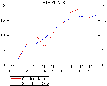
Visualization of Data

Why are the values yvals((i-n:i+n),i-n, i+n) passed to the function smooth?

What is the advantage of having a file that indicates the number of items to be read?

EXERCISES

1. Rewrite the gestation program to include functions that

sorts the gestation period array and the life span array;
calculates the gestation period array median and life span array median; and,
calculates the gestation period array mean and life span period array mean.

2. Program - Escape Velocity

Problem Definition

Interspacial travel will require a spacecraft to reach escape velocity, the velocity that a spacecraft must reach to escape from the gravitational field of a planet and travel off into space. This program calculates the escape velocity.

Input/Output Description

The input will consist of the planetary mass and radius. The following table gives the data for three planets.

**Table 2: Planet Data**
Planet	Mass (kg)	Radius (m)
Earth	6.0e24	6.4e6
Moon	7.4e22	1.7e6
Jupiter	1.9e27	7.1e7

The output is the escape velocity.

Mathematical Equation

The escape velocity is given by the expression

where G is the gravitational constant

M is the mass of the planet (in kg) and R is the planet's radius (in meters).

Algorithm

1. Prompt for and get the planetary mass and radius.

2. Write a function that uses the mass and radius to calculate the escape velocity.

3. Display the escape velocity.

Execute the program and enter the mass and radius values for Earth.

Did you get the results you expected for the escape velocity of Earth? Is it a reasonable value for the escape velocity?

Modify the escape velocity program in the following way:

use one character array for the planets' name, one real array for the mass, and one real array for the radius;
use your Internet resources to locate the mass and radius of each of the planets;
use a loop to process the data;
write the output to a file;
visualize your results by displaying your data in a bar graph.

3. Modify the Smoothing an Ordered Set of Values Program in the following way:

add 10 more data points;
add a loop that causes the data to be "smoothed" more than once during one execution of the program.

Execute the program with different values for n. How does the output differ?

Execute the program with different final values in the loop that causes the data to be smoothed more than once during one execution. How does the output differ?

4. Sinusoidal Curve Data Program

Problem Description

A sinusoidal curve, that is, a continuous curve that oscillates periodically between maximum and minimum values, is found in several real-world situations in which a dependent variable repeats its values at regular intervals as the independent variable changes. Sun spot cycles, tidal waves, sound waves, and electrical current and voltage are examples of sinusoidal curves.

The values for points that form a sinusoidal curve are specified in a table. Using the running average technique, write a program that smooths the Y values. Plot the points for each set of data on the same grid and compare the resulting curves.

Input/Output Description

The input is a data file containing the 50 original y values. The user inputs the number of values to be averaged.

The output is a graph that plots the original points and the points with the smoothed y values.

Mathematical Equations

The y values are smoothed by averaging each y value with the n proceeding and the n following y values.

Algorithm

1. Open the file and read the y values into an array called yvals.

2. Prompt for and get the number of preceding and following y values to be used for averaging (n).

3. Invoke the function that averages the y values.

4. In the function, average n proceeding y values, n following y values, and the current y value to calculate the new y value.

5. Smooth the data more than once.

6. Display the new y values and write them to a file.

7. Graph the original points and the points with the smoothed y values on the same coordinate grid.

Execute the program with different values of n and graph the results of each.

What happens to the amplitude of the curve as n increases?